In the coalescent, copies of genetic elements are traced back in time to form a genealogy of the elements that describes their ancestor and descendent relationships. In this genealogy, each time two elements have a common ancestor their lineages join to form one ancestral lineage. This event is called a coalescent event, in which two descendent lineages coalesce into one ancestral lineage in a process moving from the present into the past. The patterning of coalescent events in time provides information about the past dynamics of a population, such as fluctuations in population size or migration.

Under the Kingman n-coalescent model (Kingman 1982a; 1982b), a sample of size n is taken from a population N and the genealogy of the n individuals is traced as they coalesces back in time until they reach their most recent common ancestor (MRCA, see Figure 1)  This process involves n-1 coalescent events (i.e., events connecting two descendent lineages) going backward in time. Any two lineages may coalesce, and they do so at a per generation rate inversely proportional to the size of the population, 1/2N for diploids (1/N for haploids), adjusted by the possible pairs of lineages [k (k – 1) / 2 for k lineages]. Intuitively, large populations contain many distantly related individuals and thus have low rates of coalescence, whilst small populations contain closely related individuals and thus have high rates of coalescence.

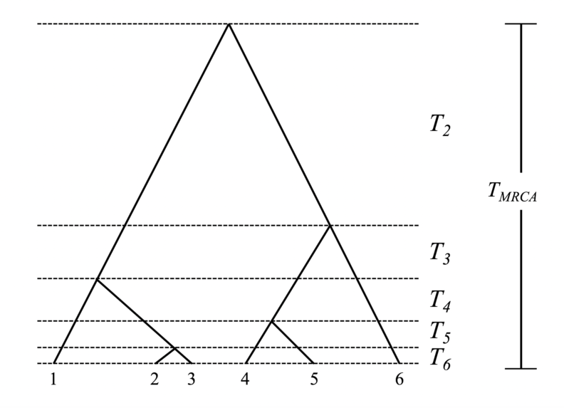
The coalescent events define a branching tree of relationships between the n individuals called a genealogy or coalescent tree. Associated with the genealogy are n-1 time intervals T_i between coalescent events. These intervals represent the waiting time for subsequent coalescent events, and their duration varies inversely with the rate of coalescence (i.e., the higher the rate the shorter the waiting time). Collectively, these intervals sum to the time of most recent common ancestry (T_MRCA), which is how long in the past the MRCA of the sample lived. Here is a representative genealogy for a sample size of n=6 with waiting times indicated:

Kingman (1982a; 1982b) demonstrated that as N tends to very large values, the coalescent intervals T_i are independent and exponentially distributed, and coalescence can be modeled as a Poisson process with rate k (k – 1) / 4N for diploids. This indicates the first coalescent event before the present should occur relatively quickly and that the last two lineages should take the longest time to coalesce. Because the T_i intervals are independent and exponentially distributed (though not identically distributed), calculating the time to the MRCA (T_MRCA), one of the most interesting parameters of a population, straightforward, and relatively easy. A classic result of coalescent theory is that T₂ (the interval directly prior to the MRCA during which there are only two lineages) is on average 2N generations for diploid populations (it is 1N generations for haploids). The expected T_MRCA for a large sample of diploids is 4N generations (it is 2N for haploids). You will notice that the times referred to above are in generations, and that time moves backward into the past; this is because the coalescent is a continuous approximation of a discrete descendent-ancestor process that occurs by tracing ancestry from the individuals in the sample to their common ancestors’ generations in the past.

Another key feature of the coalescent is that every possible coalescent tree is equally probable, as any two individuals have an equal probability of coalescing at every event. That every tree is a possible genealogy poses a challenge for relatively large datasets. For example, there are more than 2 million possible unrooted trees given 10 individuals; this number rises to more than 2.5 billion when considering rooted trees with ordered coalescent events (i.e., coalescent trees) (Edwards 1970; Wakeley 2009). Therefore, the analysis of realistically sized data sets requires a way to focus on the genealogies that contribute the most likelihood (i.e., contribute the most information about the demographic process). Genetic data may be used to identify these most probable genealogies. It is here that techniques borrowed from phylogenetic analysis can be employed to determine the set of genealogies most consistent with the data (and thus with the largest P(D|M), or likelihood). The genealogies with the greatest likelihood are those that contribute the most to inferences about the underlying demographic process, and thus focusing on these genealogies is one way to sort through the huge number of possible genealogies.

There are several key assumptions that must be made when considering the coalescent. These assumptions directly affect the shape of genealogies by distorting them from their expected distributions. This is critical, as the coalescent is powerful as a method for inferring aspects of a population from the shape of the genealogical process, so violations of these assumptions will bias inferences of a population’s demographic history. Some of these assumptions include the neutrality of genetic elements under study, no population subdivision (and no migration), constant population size over time, and the absence of recombination within the genetic locus under study (Wakeley 2009). There are extensions of the basic coalescent that include these features into the coalescent framework; the ability of the basic coalescent model to be extended to allow for a variety of demographic and evolutionary scenarios is a strength of coalescent theory.