As full-genome sequencing becomes the norm, and sampling of previously underrepresented human populations is underway, our ability to answer questions about human origins will continue to remain limited by computational power. The advantage of Bayesian inference over traditional likelihood estimation is the possibility of incorporating prior information formally into the calculations of probability. As priors simplify the calculations of the likelihood function, they reduce computational overhead. However, as the questions of human origins and history become more complex, so do the models necessary to provide answers. Bayesian inference still relies on the resolution of likelihood functions, which tend to become computationally intractable as model complexity increases (Bertorelle et al. 2010; Buzbas 2015).
As an alternative when dealing with inconclusive Bayesian inference analyses, a model rejection approach called approximate Bayesian computation (ABC) has become widely adopted for its ability to infer complex models of demographic evolution (Chan et al. 2006; Ramakrishnan and Hadly 2009; Csillery et al. 2010). ABC is a likelihood-free method; it avoids solving the likelihood portion of Bayesian inference. The intuition here is that simulated data under a known random process produce distributions of parameter values which are proportional to their likelihood. It is possible to then evaluate the probability of those parameter values in explaining the data (this is the definition of the likelihood) by comparing known aspects of the simulated data to the empirical data, to create a posterior probability of parameter values (Buzbas 2015). This feature is key, as ABC is not restricted by how complex a demographic model can be. In summary, an approximation of the likelihoods is generated by comparing simulated data against empirical data, not by solving the likelihood function.
In ABC applied to genetic studies of demography, complete genealogies are simulated computationally backwards in time to produce alignments of sequences, using the coalescent model (a known random process) as a foundation. These simulations are constrained by prior input from the user (the demographic model). For example, if the user selects a constant population size model, individuals are allowed to coalesce back into a common ancestor, but the system will prevent the effective number of individuals (a combination of number of individuals and genetic variance) to drop below that of the previous generation. In such a model, mutations have a fixed probability of occurring, or conversely being eliminated through genetic drift.
Programs such as SimCOAL (Excoffier et al. 2000), Serial SimCOAL (Anderson et al. 2005), FastSimcoal (Excoffier and Foll 2011; Excoffier et al. 2013), the R package ABC (Csilléry et al. 2012), DIYABC (Cornuet et al. 2014), and BaySICS (Sandoval-Castellanos et al. 2014) facilitate the generation of simulated alignments, and, in most cases, provide tools for model fitting analysis as well. These programs allow for manipulation of parameters of interest in the simulations, such as how effective population size is thought to have changed through time. The programs also permit more complex scenarios, including purported migration to and from adjacent populations.
Once simulated data have been generated, ABC follows the same principles as any Bayesian analysis: formulating a model (a specific realization of history), the model output (the generated sequences), which are shaped by biologically likely priors, comparing the model to data (the empirical sequences), and checking their fit. In addition, comparing the data to subsequent models allows for the selection of the optimal model (Csillery et al. 2010). The model comparison method described here is not unlike how traditional tree sampling analysis works, for which genealogy comparison can become computationally intensive (the MCMC algorithm relies extensively on the ratios of likelihoods). The crux of ABC is the way in which model comparison is performed, by comparing summary statistics calculated from the simulated data and from the empirical data.
Summary statistics:
Summary statistics aim to capture the largest amount of information in the simplest possible form (Csillery et al. 2010). Importantly, different summary statistics respond differently to evolutionary processes, the most popular example being a test for demographic neutrality known as Tajima’s D (Tajima 1989), which relies on the ratio of two separate summary statistics, segregating sites (S), and the average pairwise differences (Π). Tajima’s D is useful as an estimator of deviations from neutrality, as S and Π should be equivalent under a neutral model of evolution in which effective population size remains constant. When the population undergoes strong genetic drift, rare variants are lost faster than common variants, lowering genetic diversity as measured by both S and Π, however S is reduced faster than Π. The opposite is true under population expansion. In this way, Tajima’s D can reduce genetic information into a single summary statistics that provides insight into recent demographic events such as bottlenecks, or expansions, that are very different from a history of constant population size.
Likewise, in ABC, changes in population demographic history are expected to generate specific patterns of nucleotide variation, reflected in summary statistics derived from a given genealogy. Hence, past demographic events can be inferred from these summary statistics by detecting deviation from neutrality (Chan et al. 2006; Ramakrishnan and Hadly 2009). The cornerstone of ABC analysis lies in the assumption that finding one specific genealogy that fits the data perfectly is impractical, given the limitations in computing power. However, it is possible to select a simulated genealogy (or choose the best from various simulated genealogies) which fits closely the summary statistics of the empirical data, thus reflecting the natural demographic history by approximation. The method obtained its name from this form of approximation of the likelihood distribution.
The selection of summary statistics to be used in an ABC analysis is not trivial, as each statistic is more or less susceptible to various evolutionary processes, for example FST values are useful for estimating migration between populations, but are not informative when migration is absent from a model. A first impulse might be to include any and all information possible, as even summary statistics that may not be influenced by the evolutionary process under study may add information to the model in a small way, or at the very least, they will have no impact on the analysis. This line of thought, however, is incorrect. The addition of summary statistics increases the complexity of the analysis multiplicatively; this process is known as increasing the dimensionality of an analysis (Bertorelle et al. 2010). If one considers the range of variation of all possible values of a single summary statistic as a line, then adding the range of values of a second summary statistic would create a quadrilateral (a square for simplicity), in which we search for the model which best fits our data in two dimensions. Adding a third summary statistics would create a cube, and so on. The addition of more information decreases the accuracy of our model fitting method, making discrimination between models much more difficult.
Unfortunately, there are no general principles governing the proper number summary statistics which are optimal for model discrimination (Bertorelle et al. 2010). While it is common wisdom to limit the number of statistics to two or three, and there is important literature (Chan et al. 2006; Csillery et al. 2010) on the usefulness of certain summary statistics to approach questions on various evolutionary processes (any introductory population genetics text book should address this, for example Hartl and Clark 2006), each analysis should be optimized individually to find balance between complexity and accuracy (see the section “Power analysis to optimize ABC” below).
Model fitting algorithm
Once the number and identity of appropriate summary statistics have been selected, simulations are ranked based on their closeness to the summary statistics derived from the empirical data. The most commonly used method for estimating the distance between summary statistics is a simple standardized Euclidean error:
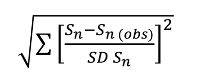
where the distance between each simulated data set and the empirical data is the normalized sum of squares of the summary statistics from a simulation (Sn) and a corresponding summary statistic drawn from the empirical data (Sn (obs)), divided by the standard deviation of the summary statistics from a simulation (SD Sn). Once a distance is associated with each simulated data set, they can be easily sorted from smallest to largest distance. Notice that typically, it is not a single simulation that is selected, but a fraction of the total simulations, from which a distribution of parameters can be generated (for example, the 1000 closest simulations), in which case, the cut-off line of accepted simulations is referred to as epsilon (ε). Epsilon is user defined.
Determining an appropriate epsilon value can be difficult, as once again there are no strict rules governing how it should be set. In most cases, epsilon is chosen independently of the distance values in the simulations themselves; instead, most choose to select a static epsilon value prior to analysis, for example, the top 0.001% of all simulations. It is informally acceptable to estimate parameter values from such a small fraction as typically the number of simulations tends to rank on a scale of 106 or larger. Of course, this can be computationally intensive as well, in which case there are other methods available for parameter estimations (see Buzbas and Rosenberg 2015).
Parameter estimation
The estimation of parameters through ABC is centered on the understanding that it is unfeasible to pin-point an exact parameter which molded the biology of the natural population under study, unless of course, all simulations are exact replicates of the observed data. Instead, by generating a distribution of parameters derived from the selected simulations by the model fitting algorithm, it is assumed that the proportion in which a parameter value occurs in the distribution reflects the likelihood of it occurring in the natural population, and thus its posterior probability (Buzbas 2015). By this understanding, parameter values can be estimated from the distribution of simulated parameters itself, which can be reported as an interval estimator (95% credibility interval is the most common), or even as a point estimate by using a mean, median or mode.
Power analysis to optimize ABC
Bayesian analyses often require extensive manipulation by the user, in the form or prior selection and study design. Similarly, the accuracy of ABC can be influenced by the choice of models simulated, the number of simulations generated, the choice of summary statistics, and by the choice of epsilon. Because of the intricacies of experimental design, it is important to generate the means to maximize the success of an analysis. Here we propose a simple method to use the simulations generated prior to model fitting as a form of statistical power analysis for the posterior distributions. The advantage of testing for statistical power previous to running an analysis on empirical data lies in the ability to modify the experimental design, either by expanding the number of simulations or adjusting the summary statistics to maximize success.
Recall that empirical data has two qualities of interest, parameters, which are unknown and to be estimated, and summary statistics, which are known. Simulated data, conversely, possesses both known parameters and known summary statistics. Therefore it is possible to treat individually simulated data as test data, which can be run through the model fitting algorithm, to produce an estimated parameter which can be scored against the known parameters of the test data, and thus ascertain the accuracy of the analysis.
As a further, and perhaps more significant advantage of posterior power analysis, is to observe the limits of ABC inference. In practical terms, genetic data may be of limited information, in either too few individuals or too few polymorphisms permit convergence on an acceptable answer. By definition, ABC will provide a parameter estimator approximated from the simulated distribution, however, it is entirely possible that this estimate is inaccurate, as several possible simulated parameters can result on similar genealogies during the coalescent process. In addition, computational resources can be limiting and prior testing can determine if a sufficient number of simulations have been generated, but more importantly, if expending resources generating further simulations is likely to increase statistical power.
Approximate Bayesian computation applied to the study of population demography based on genetic data is particularly powerful:
- It can infer complicated models of evolution from small empirical sample sets by approximating the computation of intractable likelihoods.
- It can reduce complex empirical data into summary statistics, which are then easily comparable by means of a standardized Euclidean distance.
- Prior distributions are created in the form of user-generated simulations of genealogies under various evolutionary models.
- A posterior distribution is generated by compiling the parameters from the simulations with closest Euclidean distances to the empirical data. The proportion of simulations used to generate the posterior distribution, or Epsilon, is user-defined.
- Once more, a good prior selection is fundamental to ensure convergence on an adequate solution. The implementation of an accompanying statistical power analysis such as the one presented in this review is recommended.
